Basics 01#

Nothing is better than a few good examples for quick start. A few super quick examples will show you how to kick start.

Fill a box#

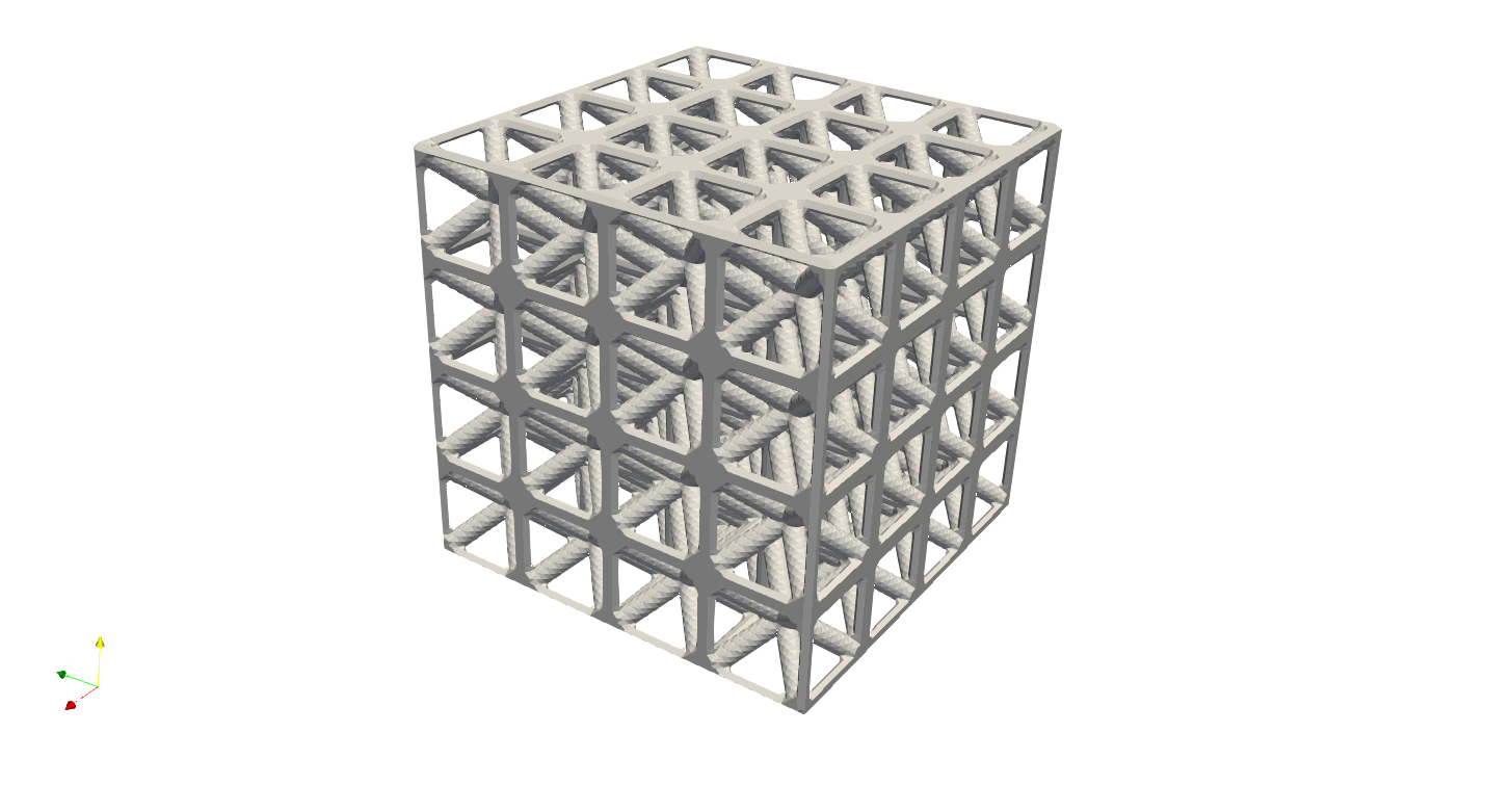
Assuming we would like to fill a box geometry with Cubic lattice, the input JSON shall be like this:

{"Setup":{  "Type" : "Sample",
            "Sample": {"Domain" : [[0.0,4.0],[0.0,4.0],[0.0,4.0]], "Shape": "Box"},
            "Geomfile": "",
            "Rot" : [0.0,0.0,0.0],
            "res":[0.05,0.05,0.05],
            "Padding": 1,
            "onGPU": false,
            "memorylimit": 1073741824000
            },
  "WorkFlow":{
      "1":{"Add_Lattice":{
                "la_name": "BCCubic", "size": [1.0,1.0,1.0], "thk":0.1, "Rot":[0.0, 0.0, 0.0], "Trans":[0.0, 0.0, 0.0],
                "Inv": false, "Fill": true, "Cube_Request": {}
                }},
       "2":{"Export": {"outfile": ".//Test_results/Test_Sample_Strut_Infill.stl"}}
       },
   "PostProcess":{"CombineMeshes": true,
            "RemovePartitionMeshFile": false,
            "RemoveIsolatedParts": false,
            "ExportLazPts": false}
}

The JSON contains three sections,

Setup, setup the general computational domain (an 3D block that computes everything) and other essential required computing quantities such as resolution (keywords res). The domain was defined in a block from (0.0,0.0,0.0) to (4.0, 4.0, 4.0) - a solid cube with length of 4 mm.
WorkFlow defines the how the resultant lattices built, e.g. connection between two different lattice fields etc.. The single step of lattice operation is defined by numeric index keywords, such as "1", "2" etc.. In the step "1", we added a BCCubic lattice with 1 mm in x, y and z direction, and the radius of the beam was 0.1 mm. In the step "2", the results saved in the file ".//Test_results/Test_Sample_Strut_Infill.stl".
PostProcess implements simple post processes on the resultant geometries. In this example, we would only combine the meshes if the automatic partitions were made.

Parameter	Details
`Type`	A string that defines how Artisan determines the computational domain. If set to `Sample`, the user must explicitly define the domain using the `Sample` parameter. If set to `Geometry`, Artisan uses the bounding box of the geometry defined by `Geomfile` as the computational domain.
`Sample`	Explicitly defines the minimum and maximum bounds of the computational domain. The format is: `{"Domain" : [[x_min, x_max], [y_min, y_max], [z_min, z_max]], "Shape": "Box"}`.
`Geomfile`	A string specifying the file path to the geometry. This geometry is considered the infill geometry, and its bounding box will be used to define the computational domain.
`Rot`	A list of three float values specifying the rotation (in degrees) applied to the imported geometry.
`Res`	A list of three float values defining the resolution of the computational domain in the X, Y, and Z directions. Smaller values result in finer triangle surfaces in the generated geometry but increase computation time.
`Padding`	Additional grid layers added around the computational domain. This value must be at least 2.
`onGPU`	A boolean flag. If set to `True`, GPU computations will be enabled. Note that not all keywords support GPU computation.
`memorylimit`	The upper limit of memory usage. Artisan will automatically partition the computational domain based on this limit.
`JsonWorkDir`	A boolean flag. If set to `True`, Artisan uses the folder containing the JSON input files as the working directory. If set to `False`, Artisan’s own folder is used. The default value is `False`. If this parameter is not specified, Artisan defaults to using its own folder. All relative paths in the `WorkFlow` procedure are resolved relative to this directory.

Save the JSON as Sample_box.json, and type

python ArtisanMain.pt -f .//Test_json//Sample_box.json

You should see the results stl file at the folder Test_results, and launch the paraview, loads the file, you should be able to see the following.

A few output files were also generated. Under the folder which contains the input JSON file, you should find the following:

“Sample_box.log”, a log file containing inputs and execution information.

“Sample_box.prg”, this is a file regularly updated during the computing procedure, it informs the current progress of percentage of job completion.

In the destination folder, you will see:

the results file, e.g. “Test_Sample_Strut_Infill.stl”, and

the partitioned mesh file “Test_Sample_Strut_Infill_000000.stl”. In this case, the partition was not triggered and only one mesh file was produced.

Two Lattices#

We certainly can add two lattice together. Artisan provides two simple connections, the hard connection - no transition between two lattice, the linear connection - a linearly changing behavior applied on two lattices.

The JSON setup below builds a cube filled with two distinct lattices, BCCubic and

{"Setup":{  "Type" : "Sample",
            "Sample": {"Domain" : [[0.0,4.0],[0.0,4.0],[0.0,4.0]], "Shape": "Box"},
            "Geomfile": "",
            "Rot" : [0.0,0.0,0.0],
            "res":[0.01,0.01,0.01],
            "Padding": 1,
            "onGPU": false,
            "memorylimit": 1073741824000
            },
 "WorkFlow":{
      "1":{"Add_Lattice":{
                "la_name": "BCCubic", "size": [1.0,1.0,1.0], "thk":0.1, "Rot":[0.0, 0.0, 0.0], "Trans":[0.0, 0.0, 0.0],
                "Inv": false, "Fill": false, "Cube_Request": {}
                }},
      "2" :{"HS_Interpolate" : {
                "la_name": "SchwarzPrimitive",
                "size": [1.0,1.0,1.0],
                "thk": 0.05, "pt":[2.0, 0.0, 0.0], "Rot":[0.0, 0.0, 0.0], "Trans":[0.0, 0.0, 0.0],
                "n_vec":[1.0, 0.0, 0.0], "Fill": true, "Cube_Request": {}
                }},
      "3":{"Export": {"outfile": ".//Test_results/Test_Sample_Strut_Infill_2lattices.stl"}}
       },
 "PostProcess":{"CombineMeshes": true,
            "RemovePartitionMeshFile": false,
            "RemoveIsolatedParts": false,
            "ExportLazPts": false}
}

You will notice it took some time to compute the results as a finer resolution was set, i.e. "res":[0.01,0.01,0.01]. The results should looks more smoother.

The keywords in "2" introduced the heaviside connection between BCCubic and the Schwarz Primitive lattice. The boundary plane is defined through the plane equation that at "pt":[2.0, 0.0, 0.0] with the normal "n_vec":[1.0, 0.0, 0.0]. The normal can be varying according to the required scenarios, it does not has to be align with axis. You could change the normal vector direction to check how it affect the combination of two lattices.

The linear varying relationship normally applied to the same lattice topological and size, but varying thickness across the regions. Let’s try the JSON below.

{"Setup":{  "Type" : "Sample",
            "Sample": {"Domain" : [[0.0,4.0],[0.0,4.0],[0.0,4.0]], "Shape": "Box"},
            "Geomfile": "",
            "Rot" : [0.0,0.0,0.0],
            "res":[0.01,0.01,0.01],
            "Padding": 1,
            "onGPU": false,
            "memorylimit": 1073741824000
            },
 "WorkFlow":{
      "1":{"Add_Lattice":{
                "la_name": "BCCubic", "size": [1.0,1.0,1.0], "thk":0.1, "Rot":[0.0, 0.0, 0.0], "Trans":[0.0, 0.0, 0.0],
                "Inv": false, "Fill": false, "Cube_Request": {}
                }},
      "2":{"Lin_Interpolate" : {
                "la_name": "BCCubic", "size": [1.0,1.0,1.0], "thk": 0.3, "Rot":[0.0, 0.0, 0.0], "Trans":[0.0, 0.0, 0.0],
                "pt_01":[0.0,0.0,0.0], "n_vec_01":[0.0,0.0,1.0],
                "pt_02":[0.0,0.0,4.0], "n_vec_02":[0.0,0.0,-1.0],
                "Inv": false, "Fill": true,
                "Cube_Request": {}
                }},
      "3":{"Export": {"outfile": ".//Test_results/Test_Sample_Strut_Infill_2lattices.stl"}}
       },
 "PostProcess":{"CombineMeshes": true,
            "RemovePartitionMeshFile": false,
            "RemoveIsolatedParts": false,
            "ExportLazPts": false}
}

The varying thickness was therefore generated from z=0.0 plane to z=4.0 plane. There is no restrictions on the plane definition. User may try change the definition and check the results.

There is a trick that the size can be varying as well, as long as the interface topology is kept. For example, the JSON below demonstrates the varying thickness and varying size of unit lattice.

{"Setup":{  "Type" : "Sample",
            "Sample": {"Domain" : [[0.0,4.0],[0.0,4.0],[0.0,8.0]], "Shape": "Box"},
            "Geomfile": "",
            "Rot" : [0.0,0.0,0.0],
            "res":[0.02,0.02,0.02],
            "Padding": 1,
            "onGPU": false,
            "memorylimit": 1073741824000
            },
 "WorkFlow":{
      "1":{"Add_Lattice":{
                "la_name": "BCCubic",
                "size": [1.0,1.0,1.0], "thk":0.1,
                "Inv": false, "Fill": false, "Rot":[0.0, 0.0, 0.0], "Trans":[0.0, 0.0, 0.0],
                "Cube_Request": {}
                }},
      "2":{"Lin_Interpolate" : {
                "la_name": "BCCubic", "size": [1.0,1.0,2.0], "thk": 0.2, "Rot":[0.0, 0.0, 0.0], "Trans":[0.0, 0.0, 0.0],
                "pt_01":[0.0,0.0,0.0], "n_vec_01":[0.0,0.0,1.0],
                "pt_02":[0.0,0.0,8.0], "n_vec_02":[0.0,0.0,-1.0],
                "Inv": false, "Fill": true,
                "Cube_Request": {}
                }},
      "3":{"Export": {"outfile": ".//Test_results/Test_Sample_Strut_Infill_2lattices.stl"}}
       },
 "PostProcess":{"CombineMeshes": true,
            "RemovePartitionMeshFile": false,
            "RemoveIsolatedParts": false,
            "ExportLazPts": false}
}

The transition cells may not be well preserved, but generally connected and is printable. In the design, user may try to keep the transition region longer, or has less dramatic change, in order to keep the shape integrity of the lattice.

../_images/Fill_box_2Lattices_Lin_VarSize.png

Attractor#

The regional thickness variation can be introduced by adding attractor operation. Attractor creates a spherical shape linearly varying field, and naturally merges this field with surrounding lattice structure. Here is an example JSON.

{"Setup":{  "Type" : "Sample",
            "Sample": {"Domain" : [[0.0,4.0],[0.0,4.0],[0.0,4.0]], "Shape": "Box"},
            "Geomfile": "",
            "Rot" : [0.0,0.0,0.0],
            "res":[0.02,0.02,0.02],
            "Padding": 1,
            "onGPU": false,
            "memorylimit": 1073741824000
            },
 "WorkFlow":{
      "1":{"Add_Lattice":{
                "la_name": "BCCubic",
                "size": [1.0,1.0,1.0], "thk":0.1, "Rot":[0.0, 0.0, 0.0], "Trans":[0.0, 0.0, 0.0],
                "Inv": false, "Fill": false,
                "Cube_Request": {}
                }},
      "2":{
      "Add_Attractor": {
                "la_name": "BCCubic",
                "size": [1.0,1.0,1.0], "thk": 0.5, "Rot":[0.0, 0.0, 0.0], "Trans":[0.0, 0.0, 0.0],
                "pt":[0.0, 0.0, 4.0], "r":3.5,
                "Inv": false, "Fill": true,
                "Cube_Request": {}
                }},
      "3":{"Export": {"outfile": ".//Test_results/Test_Sample_Strut_Infill_2lattices.stl"}}
       },
 "PostProcess":{"CombineMeshes": true,
            "RemovePartitionMeshFile": false,
            "RemoveIsolatedParts": false,
            "ExportLazPts": false}
}

In above, "pt":[0.0, 0.0, 4.0] defined the center and "r":3.5 defined the radius of the sphere. A corner of the cube has chunky material which caused by very thick beam definition, and the thickness was gradually changed and merged to the surrounding.

../_images/Fill_box_2Lattices_Attractor.png

Rotation and Translation#

To fit a design purpose, users can apply rotation and translation on the lattice unit orientation. It is important to note that only periodic lattices can be rotated and translated with respect to the global origin and axes. Currently, the following keywords support these two operations: Add_Lattice, Subtract_Lattice, HS_Interpolate, Lin_Interpolate, Add_Attractor, and OP_FieldMerge.

In the example JSON below, the lattice is rotated with respect to the x-axis by \(\frac{\pi}{4}\) radians.

{"Setup":{      "Type" : "Sample",
            "Sample": {"Domain" : [[0.0,4.0],[0.0,4.0],[0.0,4.0]], "Shape": "Box"},
            "Geomfile": "",
            "Rot" : [0.0,0.0,0.0],
            "res":[0.025,0.025,0.025],
            "Padding": 1,
            "onGPU": false,
            "memorylimit": 1073741824000
            },
"WorkFlow":{
      "1":{"Add_Lattice":{
                "la_name": "Cubic", "size": [1.0,1.0,1.0], "thk":0.05,
                "Rot":[0.7853981633974483, 0.0, 0.0], "Trans":[0.0,0.0,0.0], "Inv": false, "Fill": true,
                "Cube_Request": {}
                }},
      "2":{"Export": {"outfile": ".//Test_results/Test_Sample_Strut_Infill.stl"}}
       },
"PostProcess":{"CombineMeshes": true,
            "RemovePartitionMeshFile": false,
            "RemoveIsolatedParts": false,
            "ExportLazPts": false}
}

The parameter Rot in the keywords Add_Lattice becomes [0.7853981633974483, 0.0, 0.0]. The first element represents the rotation around x-axis in radius unit, and the second and third element defines the y- and z-axis rotation. Same setup applies to the Trans that defines the translation movement. It has to note that, Artisan rotates the lattice before translating it.

User may define the parameter Trans to get after rotation translation, for instance, move the structure by 0.5 in x direction "Trans":[0.5, 0.0, 0.0].

Basics 01

Contents

Basics 01#

Fill a box#

Two Lattices#

Attractor#

Rotation and Translation#