Lattice Transition#
Design a lattice fill often means a combination of various styles and sizes across different parts of the component. The transition amongst these regional features could be a challenge task. Artisan is capable of automatically merging different lattice designs through the field based morphing algorithm.
Artisan treats the regional lattice designs as various fields, and the fields can be interpolated through certain mathematical ways, for example, a regional attractor or linearly interpolating between two lattices. Here we use a few simple examples to demonstrate the applications. User may find these examples under the folder \Test_json\FieldMerge\.
Simple Transition#
Considering to fill a bar region with two different lattices, BC on one side gradually transits to the other side and merged with BCCubic lattice, see the JSON below.
{"Setup":{  "Type" : "Sample",
            "Sample": {"Domain" : [[0.0,100.0],[0.0,30.0],[0.0,30.0]], "Shape": "Box"},
            "Geomfile": "",
            "Rot" : [0.0,0.0,0.0],
            "res":[0.5,0.5,0.5],
            "Padding": 1,
            "onGPU": false,
            "memorylimit": 1073741824000
            },
 "WorkFlow":{
      "1": {"Add_Lattice":{
                "la_name": "BC", "size": [10.0,10.0,10.0], "thk":1.2, "Rot":[0.0, 0.0, 0.0], "Trans":[0.0, 0.0, 0.0],
                "Inv": false, "Fill": false, "Cube_Request": {}
                }
           },
      "2":{"OP_FieldMerge":{ "la_name":"BCCubic", "size":[10.0,10.0,10.0], "thk":1.2, "Rot":[0.0, 0.0, 0.0], "Trans":[0.0, 0.0, 0.0],
                             "OP_para":{
                                        "InterpType": "Linear",
                                        "pt_01":[10.0,0.0,0.0], "n_vec_01":[ 1.0,0.0,0.0],
                                        "pt_02":[90.0,0.0,0.0], "n_vec_02":[-1.0,0.0,0.0],
                                        "Transition": {}
                                        },
                             "Fill":true, "Cube_Request": {}
                                                       }
          },
      "3":{"Field_Boundary": {"Boundary": "Box"}},
      "4":{"Export": {"outfile": ".//Test_results/Box_FieldMerge_Lin.stl"}}
       },
 "PostProcess":{"CombineMeshes": true,
                "RemovePartitionMeshFile": false,
                "RemoveIsolatedParts": false,
                "ExportLazPts": false}
}
The item "2" keywords OP_FieldMerge in WorkFlow defines the field base lattice transition. It is similar to the keywords Lin_Interpolate which requires a definition of second field (an added on field), here the lattice field BCCubic. OP_para contains the parameters for calculating the transition of the geometric features.
|
Defines the plane that starts the transition from the main field. |
|---|---|
|
Defines the plane that ends the transition at the second field. |
|
This parameter defines the influence lattice that used to guide the transition between two fields. If it is empty, no transition computation will be initiated. |
Note
Artisan 0.1.10 and later version does NOT require nJobs and ScratchPath parameters for the keywords OP_FieldMerge. Historically nJobs defines the number of parallel threading used for computation. If it is 0 or negative number, it will use all available resources, if 1, normal serial computation. ScratchPath defines the working folder for exchange of data during parallel computation.
The transition of two lattices should be looks like below. The vertical and horizontal beams were gradually growing until merged together.

Like many algorithm, the plain transition may not produce a “perfect” results. For instance, below shows a case that BC lattice transiting to the Cubic lattice.

The transition was mathematically right, but the resultant geometry had a large number of floating bits and the connectivity was broken at the middle part. In order to ensure the transition with good connectivity, Transition parameter is introduced. The JSON below shows the connected transition between BC and Cubic through a bridging lattice BCCubic.
{"Setup":{      "Type" : "Sample",
            "Sample": {"Domain" : [[0.0,100.0],[0.0,30.0],[0.0,30.0]], "Shape": "Box"},
            "Geomfile": "",
            "Rot" : [0.0,0.0,0.0],
            "res":[0.5,0.5,0.5],
            "Padding": 1,
            "onGPU": false,
            "memorylimit": 1073741824000
            },
 "WorkFlow":{
      "1": {"Add_Lattice":{
                "la_name": "BC", "size": [10.0,10.0,10.0], "thk":1.2, "Rot":[0.0, 0.0, 0.0], "Trans":[0.0, 0.0, 0.0],
                "Inv": false, "Fill": false, "Cube_Request": {}
                }
           },
      "2":{"OP_FieldMerge":{ "la_name":"Cubic", "size":[10.0,10.0,10.0], "thk":1.2, "Rot":[0.0, 0.0, 0.0], "Trans":[0.0, 0.0, 0.0],
                             "OP_para":{
                                        "InterpType": "Linear",
                                        "pt_01":[10.0,0.0,0.0], "n_vec_01":[ 1.0,0.0,0.0],
                                        "pt_02":[90.0,0.0,0.0], "n_vec_02":[-1.0,0.0,0.0],
                                        "Transition": {"la_name":"BCCubic", "size":[10.0,10.0,10.0], "thk":1.2, "Weight": 0.2, "f_trans":0.15}
                                        },
                             "Fill":true, "Cube_Request": {}
                                                       }
          },
      "3":{"Field_Boundary": {"Boundary": "Box"}},
      "4":{"Export": {"outfile": ".//Test_results/Box_FieldMerge_Lin.stl"}}
       },
 "PostProcess":{"CombineMeshes": true,
            "RemovePartitionMeshFile": false,
            "RemoveIsolatedParts": false,
            "ExportLazPts": false}
}
The parameter Transition contains the following parameter to setup the bridging lattice field.
|
Defines the bridging lattice design. |
|---|---|
|
Defines the influence factor of the third field on the transition calculation. |
|
Defines the transition rate of the bridging lattice towards the main lattice and the second lattice; if it is less than |

The BC lattice transformed to Cubic field through bridging lattice BCCubic. User may try different Weight and f_trans to check how the factors affect the results.
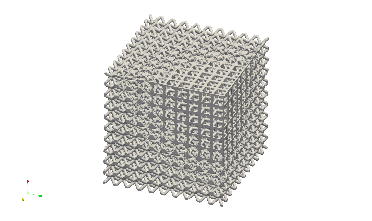
In addition to Linear transition, OP_FieldMerge supports Attractor transition which is similar to the keywords Add_Attractor. The JSON below demonstrates the merging of Cubic lattice with regionally varying size.
{"Setup":{  "Type" : "Sample",
            "Sample": {"Domain" : [[0.0,100.0],[0.0,100.0],[0.0,100.0]], "Shape": "Box"},
            "Geomfile": "",
            "Rot" : [0.0,0.0,0.0],
            "res":[0.5,0.5,0.5],
            "Padding": 1,
            "onGPU": false,
            "memorylimit": 1073741824000
            },
 "WorkFlow":{
      "1": {"Add_Lattice":{
                "la_name": "Cubic", "size": [10.0,10.0,10.0], "thk":1.2, "Inv": false, "Fill": false,
                "Cube_Request": {}
                }
           },
      "2":{"OP_FieldMerge":{ "la_name":"Cubic", "size":[5.0,5.0,5.0], "thk":1.2, "Rot":[0.0, 0.0, 0.0], "Trans":[0.0, 0.0, 0.0],
                             "OP_para":{
                                        "InterpType": "Attractor",
                                        "pt_att": [100.0,100.0,100.0],
                                        "pt_r": 125.0,
                                        "Transition": {}
                                       },
                             "Fill":true, "Cube_Request": {}
                                                       }
          },
      "3":{"Field_Boundary": {"Boundary": "Box"}},
      "4":{"Export": {"outfile": ".//Test_results/Box_FieldMerge_VarSize.stl"}}
       },
 "PostProcess":{"CombineMeshes": true,
            "RemovePartitionMeshFile": false,
            "RemoveIsolatedParts": false,
            "ExportLazPts": false}
}
The parameter pt_att defines the coordinate of the attractor, and pt_r defines the radius of the ball which covers the whole transition. The results are shown below. User may find the complete JSON in the file Box_FieldMerge_Attractor.json.


The third option is the Annulus transition. It defines the inner radius and outer radius, and the transition happens between-in the range of annulus area. User may find the example file Box_FieldMerge_Annulus.json.
{"Setup":{    "Type" : "Sample",
              "Sample": {"Domain" : [[0.0,100.0],[0.0,100.0],[0.0,100.0]], "Shape": "Box"},
              "Geomfile": "",
              "Rot" : [0.0,0.0,0.0],
              "res":[0.5,0.5,0.5],
              "Padding": 1,
              "onGPU": false,
              "memorylimit": 1073741824000
              },
 "WorkFlow":{
        "1": {"Add_Lattice":{
                  "la_name": "BC", "size": [10.0,10.0,10.0], "thk":1.2, "Rot":[0.0,0.0,0.0], "Trans":[0.0,0.0,0.0], "Inv": false, "Fill": false,
                  "Cube_Request": {}
                  }
             },
        "2":{"OP_FieldMerge":{ "la_name":"Cubic", "size":[10.0,10.0,10.0], "thk":1.2, "Rot":[0.0,0.0,0.0], "Trans":[0.0,0.0,0.0],
                               "OP_para":{
                                          "InterpType": "Annulus",
                                          "pt_att": [100.0,100.0,100.0],
                                          "inner_r": 40.0,
                                          "outer_r": 100.0,
                                          "Transition": {"la_name":"BCCubic", "size":[10.0,10.0,10.0], "thk":1.2, "Weight": 0.8, "f_trans":0.5}
                                          },
                               "Fill":true, "Cube_Request": {}
                                                         }
            },
        "3":{"Field_Boundary": {"Boundary": "Box"}},
        "4":{"Export": {"outfile": ".//Test_results/Box_FieldMerge_AnnulusAttractor.stl"}}
         },
 "PostProcess":{"CombineMeshes": true,
              "RemovePartitionMeshFile": false,
              "RemoveIsolatedParts": false,
              "ExportLazPts": false}
}
The above JSON produce the result below. The inner radius defined a large area filled with Cubic lattice, where as the transition area becomes smaller compared with previous case. Larger transition area shall give better shape continuity.
Field Based Transition#
The physical quantities, such as stress, strain, and force, or other field can serve as external design parameters influencing the lattice transition. Similar to field operations, the keyword OP_FieldMerge can be employed to read a field, evaluate the target lattice, and ultimately combine the current field with the global field. This merging operation is demonstrated using the bar model case - the same example from the field operation section. This example īs the file Bar_FieldMerge_Field.json.
{"Setup":{  "Type" : "Geometry",
            "Geomfile": ".//sample-obj//Bar//Bar.stl",
            "Rot" : [0.0,0.0,0.0],
            "res":[0.5, 0.5, 0.5],
            "Padding": 1,
            "onGPU": false,
            "memorylimit": 16106127360
              },
  "WorkFlow":{
          "1": {"Add_Lattice":{
              "la_name": "BC", "size": [25.0, 25.0, 25.0], "thk":2.5, "Rot":[0.0,0.0,0.0], "Trans":[0.0,0.0,0.0], "Inv": false, "Fill": true,
              "Cube_Request": {}
              }
              },
          "2":{"OP_FieldMerge":{  "la_name":"BCCubic", "size":[25.0, 25.0, 25.0], "thk":2.5,
                                  "Rot":[0.0,0.0,0.0], "Trans":[0.0,0.0,0.0],
                                  "OP_para":{
                                          "InterpType": "Field",
                                          "FieldFile": ".//sample-obj//Bar//fielddata.csv",
                                          "max_cap": 4500000,
                                          "min_cap": 3500000,
                                          "Transition": {}
                                          },
                                "Fill":true, "Cube_Request": {}
                                                         }
            },
          "3":{"Field_Boundary": {"Boundary": "Box"}},
          "4":{"Export": {"outfile": ".//Test_results/Bar_FieldMerge_Field.stl"}}
         },
    "PostProcess":{"CombineMeshes": true,
              "RemovePartitionMeshFile": false,
              "RemoveIsolatedParts": true,
              "ExportLazPts": false}
  }
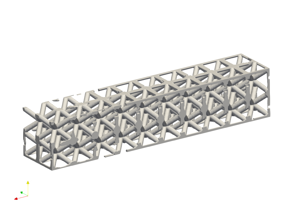
The above JSON produce the following simple transition between BC and BCCubic lattice. The keyword OP_FieldMerge has new OP_Para parameter "InterpType": "Field", and the lattice transition occurs within the range specified by max_cap and min_cap.
Parameter |
Details |
|---|---|
|
CSV file, has same file format to the field operation |
|
the maximum capped value in the given field, any spatial points with higher value will be considered as target lattice occupied area; |
|
the minimum capped value in the given field, any spatial points with higher value will be considered as current lattice occupied area; |
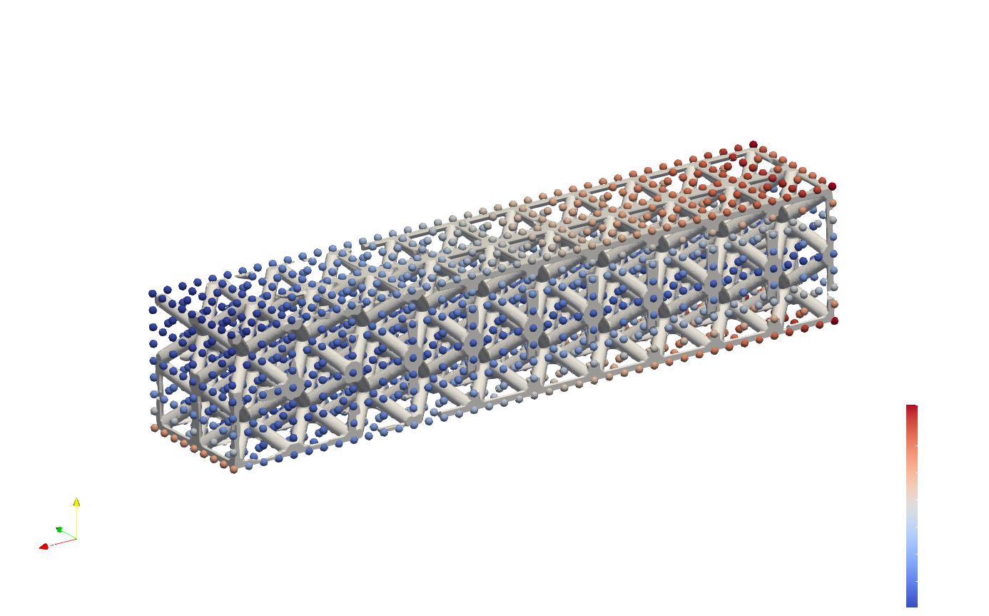
The results, depicted below, illustrate that the lattice transition progresses along the X-axis. The cubic-like lattice gradually transforms into a BC-like lattice. When overlaid with the given field, the results indicate that the high-temperature area also aligns with the X-axis. This transition effectively adheres to a simple logic that the material is only added to areas with higher field values.
Transition on Conformal Lattices#
The transition supports all lattice definitions in all circumstances. In other words, the lattices can be transformed to any given shape that forms a local lattice field. It would be good that two lattices share a similar geometric or topological similarity. The example below shows the transition of conformed BC lattice to the conformed box-frame object lattice in a twisted bar geometry. Two lattices have similar shape features, however, with many different details.
{"Setup":{      "Type" : "Geometry",
            "Geomfile": ".//sample-obj//Twisted_Bar//Twisted_Bar.stl",
            "Rot" : [0.0,0.0,0.0],
            "res":[3.0,3.0,3.0],
            "Padding": 3,
            "onGPU": false,
            "memorylimit": 16106127360
            },
"WorkFlow":{
      "1": {"Add_Lattice":{
                "la_name": ".//Test_json//LatticeMerge//Twisted_Bar_Conformal_La01.mld",
                "size": [200.0,200.0,200.0], "thk":5.0, "Inv": false, "Fill": false,
                "Cube_Request": {}
                }
           },
              "2":{"OP_FieldMerge":{ "la_name":".//Test_json//LatticeMerge//Twisted_Bar_Conformal_La02.mld",
                             "size":[200.0,200.0,200.0], "thk":15.0, "Rot":[0.0, 0.0, 0.0], "Trans":[0.0, 0.0, 0.0],
                             "OP_para":{
                                        "InterpType": "Linear",
                                        "pt_01":[300.0,0.0,0.0], "n_vec_01":[ 1.0,0.0,0.0],
                                        "pt_02":[900.0,0.0,0.0], "n_vec_02":[-1.0,0.0,0.0],
                                        "Transition": {}
                                        },
                             "Fill":false, "Cube_Request": {}
                                                       }
          },

      "3":{"Export": {"outfile": ".//Test_results/Twisted_Bar_ConformalCustomLattice.stl"}}
       },
"PostProcess":{"CombineMeshes": true,
            "RemovePartitionMeshFile": false,
            "RemoveIsolatedParts": false,
            "ExportLazPts": false}
}
The conformal lattice definition in Twisted_Bar_Conformal_La01.mld:
{
 "type": "ConformalLattice",
 "definition": {
       "meshfile": ".//sample-obj//Twisted_Bar//Twisted_Bar.med",
       "la_name" : ".//Test_json//LatticeMerge//CustomLattice_Geom.txt"
        }
}
and CustomLattice_Geom.txt defines
{
 "type": "Geom",
 "definition": {
       "file": ".//sample-obj//boxframe.obj",
       "ladomain": "Hex"}
}
The second lattice definition in Twisted_Bar_Conformal_La02.mld setup the Cubic lattice.
{
 "type": "ConformalLattice",
 "definition": {
        "meshfile": ".//sample-obj//Twisted_Bar//Twisted_Bar.med",
        "la_name" : "Cubic"
        }
}
The results below shows a good smooth transition from a customer defined geometric lattice to a beam-like Cubic lattice.


Here are a few hits and keypoints of using OP_FieldMerge algorithm:
The best pairing of two merged lattices shall have some topological similarities. This ensures a smooth and continuously connected transition.
The bridging lattice has to be considered to assist the lattices which have no close topological or geometric similarity.
User may requires standard shape cases studies, e.g. on the box or bar shape, to check the lattice transition before applying to actual design.
The computation of the merging algorithm is heavy, and requires longer time to finish the task. User shall expect a long computation time on the complex design.
Increasing the resolution, or the transition region, may improve the continuous connectivity of the lattice, however, this could yield a longer computation time.