Line Structure 01#

Line structures that conform to complex shapes can be generated without explicitly defining lattice units or meshes. Artisan currently supports two primary approaches for constructing line structures: point-based algorithms and field-based generation. The point-based approach uses specialized algorithms to connect predefined material points, while the field-based approach allows users to leverage external fields, internal fields, and Artisan’s grid field container to build a target field and generate line structures directly from it. Future development will focus on expanding and integrating more advanced line structure generation capabilities within Artisan.

Minimum Spanning Tree#

A Minimum Spanning Tree (MST) is a graph-based optimization method used to connect a set of points with the minimum total connection cost. In a connected, weighted, undirected graph, an MST links all vertices together without forming cycles while minimizing the sum of edge weights. This makes it an efficient solution for designing lightweight networks, such as transportation systems, communication networks, and structural frameworks. In computational design, MST algorithms can be used to generate optimized line structures by efficiently connecting material points while reducing redundancy.

Example .//Test_json//MaterialPoints//BingDunDun_Infill_LR.json gives a basic workflow of generating MST line structure.

    {
    "Setup": {
        "Type": "Geometry",
        "Sample": {
            "Domain": [
                [0.0, 0.0],
                [0.0, 0.0],
                [0.0, 0.0]
            ],
            "Shape": "Box"
        },
        "Geomfile": ".//sample-obj//shell_1_of_bdd_.stl",
        "Rot": [0.0, 0.0, 0.0],
        "res": [0.8, 0.8, 0.8],
        "Padding": 1,
        "onGPU": false,
        "memorylimit": 161061273000
    },
    "WorkFlow": {
        "1": {
            "Gen_MaterialPoints_SurfaceLayers":{
                "inp_meshfile":".//sample-obj//shell_1_of_bdd_.stl",
                "depth": [0, 10],
                "res":[5.0, 5.0, 1.8],
                "sampling": "Poisson",
                "out_matpoints_file": ".//Test_results//BingDunDun_MatPts_Grid.csv"
            }
        },
        "2": {
            "Gen_MSTMesh_Basic":{
                "inp_matpoints_file":".//Test_results//BingDunDun_MatPts_Grid.csv",
                "out_meshfile":".//Test_results//BingDunDun_MST_Mesh.inp"
            }
        },
        "3":{
            "Define_Lattice":{
                "la_name": "MSTMesh",
                "definition":{
                    "type": "MeshLattice",
                    "definition": {
                        "meshfile": ".//Test_results//BingDunDun_MST_Mesh.inp"
                    }
                }
            }
        },
        "4": {"Add_Lattice":{
                    "la_name": "MSTMesh",
                    "size": [5.0,5.0,5.0], "thk":1.2, "Rot":[0.0,0.0,0.0], "Trans":[0.0,0.0,0.0], "Inv": false, "Fill": false,
                    "Cube_Request": {}
                    }
               },
        "5":{
              "Export": {"outfile": ".//Test_results//BingDunDun_MST_Lattice.stl"}
              }

    },
    "PostProcess": {
        "CombineMeshes": true,
        "RemovePartitionMeshFile": false,
        "RemoveIsolatedParts": true,
        "ExportLazPts": false
    }
}

Above workflow does the following operations.

Work item 1 with Gen_MaterialPoints_SurfaceLayers generates sampling points on the surface of geometry with 0 and 10 depth.
Work item 2 with Gen_MSTMesh_Basic computes the MST line structure with previous generated material points and export the results as beam elements.
Work item 3 with Define_Lattice defines the mesh lattice which read the mesh exported from item 2 .
Work item 4 with Add_Lattice generate the lattice.
Work item 5 with Export extracts the mesh and export the mesh into a file.

The parameters of the keyword Gen_MaterialPoints_SurfaceLayers are defined as below.

Parameter	Details
`inp_meshfile`	A file path string of the input geometry.
`depth`	A list of numerical values that defines the sampling surfaces. In this example, the material is sampled on the geometry surface itself (SDF depth `0.0`) as well as on an inward offset surface at an SDF depth of `10.0`.
`res`	approximated material points spacing distance in X, Y and Z direction.
`sampling`	Sampling strategy, it supports `Poisson` sampling algorithm in the current version.
`out_matpoints_file`	the export file path of the generated material points.

The parameters of the keyword Gen_MSTMesh_Basic are defined as below.

Parameter	Details
`inp_matpoints_file`	A file path string of the input material points file.
`out_meshfile`	an exported results mesh file, or mesh id in mesh container.

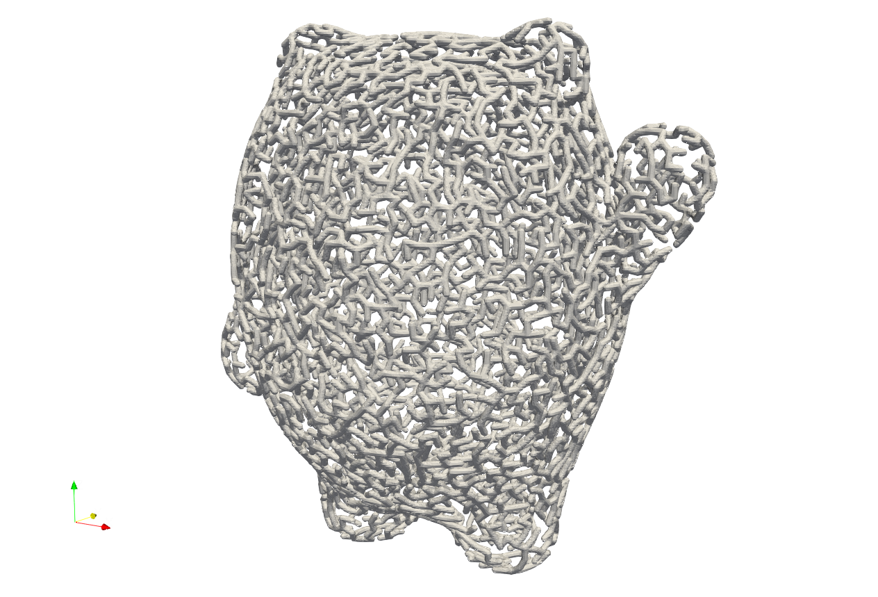
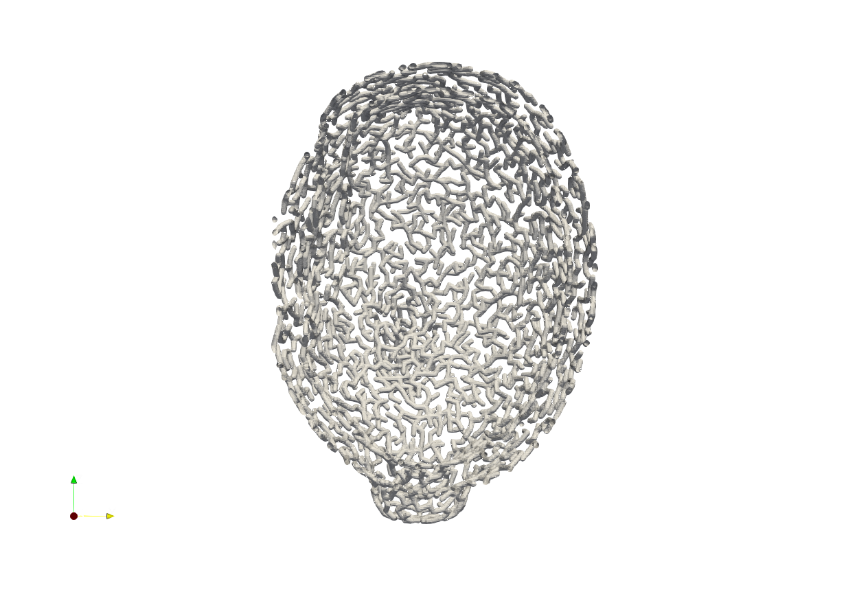
Two layers of tree structures were generated based on defined depth.

Streamlines over Field#

Artisan is now focusing on the development of field based line structure without defining mesh and lattice unit. Unlike the mesh based conformal lattice, the field based line structure lattice do not rely on the pre-defined mesh, or lattice unit, user only need to produce a field that conformal to the geometry shape, and use the streamline algorithm to generate the structure.

Example Test_jsonLaplaceFieldLaplaceField_LineStructure.json shows a procedure of field based conformal line structure lattice generation using laplace field.

{
"Setup": {
    "Type": "Geometry",
    "Sample": {
        "Domain": [
            [0.0, 0.0],
            [0.0, 0.0],
            [0.0, 0.0]
        ],
        "Shape": "Box"
    },
    "Geomfile": "..//..//sample-obj//LaplaceFieldGeometry.stl",
    "Rot": [0.0, 0.0, 0.0],
    "res": [1.0, 1.0, 1.0],
    "Padding": 5,
    "onGPU": false,
    "memorylimit": 161061273000,
    "JsonWorkDir": true
},
"WorkFlow": {
    "1": {
        "Gen_Field_Laplace": {
            "inp_meshfile":"..//..//sample-obj//LaplaceFieldGeometry.stl",
            "res": [2.5, 2.5, 2.5],
            "sources":[75.0, 75.0, 170.0],
            "source_strengths":[1000.0],
            "sinks":[75.0, 75.0, -35.0],
            "sink_strengths": [-1000.0],
            "influence_factors": {
                "radius": 50,
                "kernel": "tophat"
            },
            "solver_factors":{
                "method": "bicgstab",
                "tol": 1e-3,
                "maxiter":300
            },
            "out_fieldfile": "LaplaceField",
            "is_create_on_lattice_field": false
        }
    },
    "2":{
        "Gen_Mesh_Streamlines": {
            "inp_fieldfile":"LaplaceField",
            "out_meshfile":"..//..//Test_results//LaplaceField_Mesh.inp",
            "source": [75.0, 75.0, 170.0],
            "sink": [75.0, 75.0, -35.0],
            "step": 1.5,
            "num_integration_steps": 350,
            "num_streamlines_seeds": 100,
            "source_plane_dir": [0.0, 0.0, -1.0],
            "source_plane_radius": 20.0,
            "min_streamlines_spacing": 2.0
        }
    },
    "3": {
    "Define_Lattice":{
        "la_name": "LaplaceStreamLines",
        "definition": {
                "type": "MeshLattice",
                "definition": {
                        "meshfile": "..//..//Test_results//LaplaceField_Mesh.inp",
                        "k" : 0.0
                            }
                    }
                }
        },
    "4": {"Add_Lattice":{
            "la_name": "LaplaceStreamLines",
            "size": [10.0,10.0,10.0],
            "thk":1.2, "Rot":[0.0, 0.0, 0.0], "Trans":[0.0, 0.0, 0.0],
            "Inv": false, "Fill": true, "Cube_Request": {}
            }
       },
    "999":{"Export": {"outfile": "..//..//Test_results//LaplaceField_LineMeshLattice.stl"}}
},
"PostProcess": {
    "CombineMeshes": true,
    "RemovePartitionMeshFile": false,
    "RemoveIsolatedParts": true,
    "ExportLazPts": false
    }
}

Above workflow does the following operations.

Work item 1 with Gen_Field_Laplace solves the laplace equation with defined source and sink points.
Work item 2 with Gen_Mesh_Streamlines reads the field, and generates the streamlines of the field.
Work item 3 with Define_Lattice defines the mesh lattice which read the mesh exported from item 2 .
Work item 4 with Add_Lattice generate the lattice.
Work item 5 with Export extracts the mesh and export the mesh into a file.

The Gen_Field_Laplace keyword solves a well-defined Laplace equation over the specified domain. In this formulation, the given geometry is treated as the boundary, with a zero normal flux boundary condition applied, for example, effectively modeling the boundary as a perfectly insulated layer, analogous to a heat transfer conduction problem with no flux across the surface.

The parameters of the keyword Gen_Field_Laplace are defined as below.

Parameter	Details
`inp_meshfile`	A mesh ID or file path of defined geometry as boundary of the field problem.
`res`	A list of numerical values that defines the sampling surfaces. In this example, the material is sampled on the geometry surface itself (SDF depth `0.0`) as well as on an inward offset surface at an SDF depth of `10.0`.
`sources`	A list of 3 float numbers defining the coordinate of source.
`source_strengths`	Strength of the source, usually this is a positive number.
`sinks`	A list of 3 float numbers defining the coordinate of sink.
`sink_strengths`	Strength of the sink, usually this is a negative number.
`influence_factors`	This defines the source and sink influence volumes, it contains two parameters, `kernel` defines influence pattern, `tophat` means the strength maintaining constant value within this given `radius` volume.
`solver_factors`	This defines the solver related parameters: `method` supports the solver `cg`, `gmres`, `bicgstab`, `spsolve` and `splu`; `tol` defines tolerance of the numerical convergence; `maxiter` defines the maximum number of iteration.
`out_fieldfile`	the export ID or file path for the field results.
`is_create_on_lattice_field`	if `true`, the grids over the domain for numerical solution will created on the lattice field.

The keyword Gen_Mesh_Streamlines generates the stream lines from field as beam element based mesh. User may use this mesh as tool mesh, for example, to generate the pipe lines for fluids driven heat transferring application.

The parameters of the keyword Gen_Mesh_Streamlines are defined as below.

Parameter	Details
`inp_fieldfile`	A field ID or a field file path as input field.
`out_meshfile`	A mesh ID or mesh file path for exporting results.
`source`	A coordinate of the source point.
`sink`	A coordinate of the sink point, e.g. stop point.
`num_integration_steps`	The number of numerical integration steps.
`source_plane_dir`	The keyword will define a circle area for generating a number of seed points to start computing the stream lines, `source_plane_dir` defines the direction of plane at the `source` point.
`source_plane_radius`	The radius of the circle around the `source` point to generate the seed points.
`num_streamlines_seeds`	The total number of candidate seed points of the starting points of stream lines. Please note, the some candidates will be removed from results if neighboring two lines are smaller than the `min_streamlines_spacing`.
`min_streamlines_spacing`	minimum spacing between two neighboring stream lines, if less than, one stream line will be removed from result.

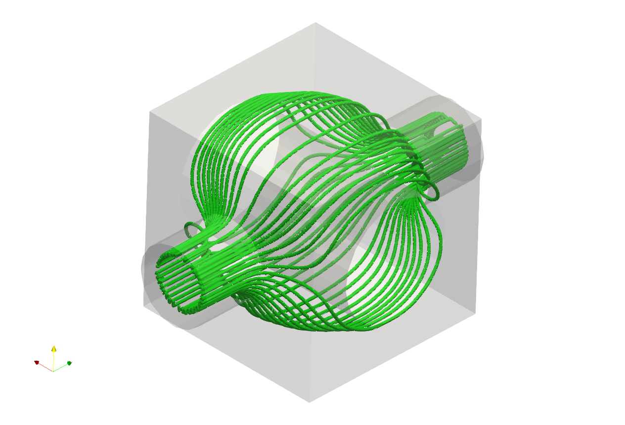
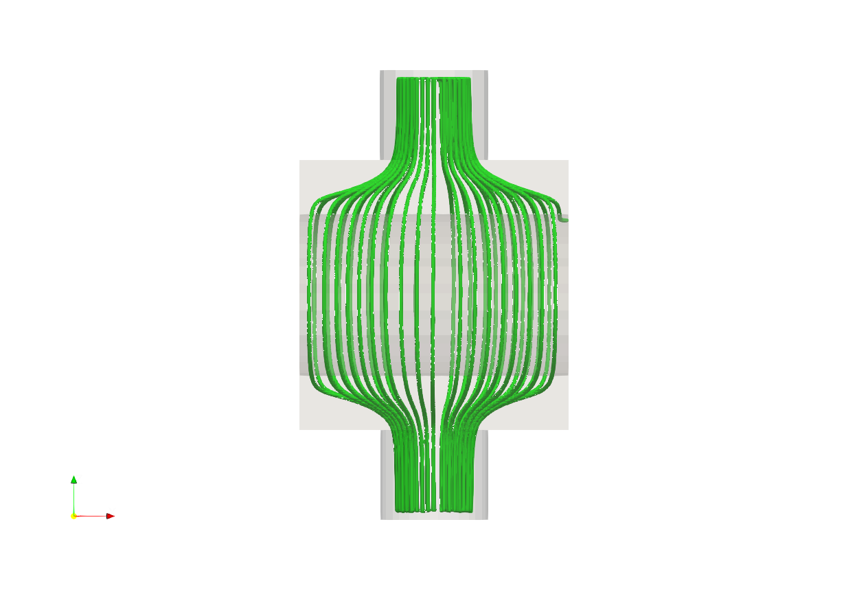
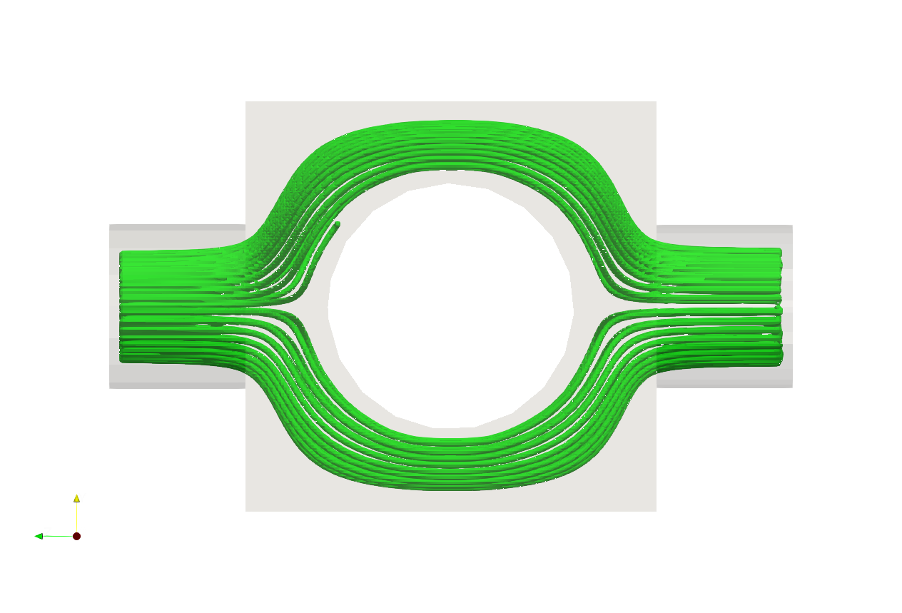
Below, the streamline lattice is overlaid within the specified geometric domain. The generated lattice, highlighted in green, conforms perfectly to the given geometry. Users can further generate multiple layers to fill the remaining available space.

Parametric Curve#

Artisan provides the keyword Gen_ParametricLineMesh to generate a line mesh from a user-defined parametric curve. The curve is defined by three mathematical expressions:

x = f(t)
y = g(t)
z = h(t)

where t is the curve parameter.

Artisan evaluates the three expressions over the specified parameter range and connects consecutive points to form line elements. This feature can be used to generate arbitrary curves, including straight lines, circular curves, helices, and other mathematical curves. A simple parametric curve can be generated using:

{
    "Gen_ParametricLineMesh": {
        "x_expr": "100*cos(t)",
        "y_expr": "100*sin(t)",
        "z_expr": "0",
        "t_min": 0.0,
        "t_max": 6.283185307,
        "n_points": 100,
        "periodic": true,
        "out_meshfile": "ParametricLine.inp"
    }
}

The above example generates a circular curve in the XY plane. The x_expr, y_expr, and z_expr parameters define the coordinates of the curve. For example:

"x_expr": "100*cos(t)",
"y_expr": "100*sin(t)",
"z_expr": "0"

defines the curve:

\[x(t) = 100\cos(t)\]

\[y(t) = 100\sin(t)\]

\[z(t) = 0\]

The parameter t is used as the curve parameter. Artisan supports common mathematical functions such as sin cos, tan, sqrt, exp, log, and abs, as well as the constants pi and e. The t_min and t_max parameters define the parameter range used to generate the curve. For example:

"t_min": 0.0,
"t_max": 6.283185307

generates the curve over the specified parameter range. The value of t_max must be greater than t_min. The n_points parameter specifies the number of points generated along the curve. For example:

"n_points": 100

generates 100 points between t_min and t_max.

Consecutive points are connected to form line segments. Therefore, for a non-periodic curve with n_points points, the generated mesh contains \(n\_points - 1\) line segments. Instead of specifying n_points, the curve can be generated using step_size. For example:

"step_size": 5.0

Artisan automatically determines the number of points from the parameter range and the specified step size. Only one of n_points or step_size is required. If n_points is provided, it is used to determine the number of points. Otherwise, step_size is used. The periodic parameter determines whether the generated curve is closed. For example:

"periodic": true

adds the starting point again at the end of the generated point sequence, closing the curve with a final line segment. This is useful for closed curves such as circles. For example:

{
    "x_expr": "100*cos(t)",
    "y_expr": "100*sin(t)",
    "z_expr": "0",
    "t_min": 0.0,
    "t_max": 6.283185307,
    "n_points": 100,
    "periodic": true,
    "out_meshfile": "Circle.inp"
}

When periodic is false, Artisan generates an open curve without adding the closing segment. Here are a few examples. A straight line along the X direction can be defined as:

{
    "x_expr": "t",
    "y_expr": "0",
    "z_expr": "0",
    "t_min": 0.0,
    "t_max": 100.0,
    "n_points": 21,
    "periodic": false,
    "out_meshfile": "StraightLine.inp"
}

A circle in the XY plane can be defined as:

{
    "x_expr": "100*cos(t)",
    "y_expr": "100*sin(t)",
    "z_expr": "0",
    "t_min": 0.0,
    "t_max": 6.283185307,
    "n_points": 100,
    "periodic": true,
    "out_meshfile": "Circle.inp"
}

A three-dimensional helix can be defined as:

{
    "x_expr": "100*cos(t)",
    "y_expr": "100*sin(t)",
    "z_expr": "10*t",
    "t_min": 0.0,
    "t_max": 12.566370614,
    "n_points": 200,
    "periodic": false,
    "out_meshfile": "Helix.inp"
}

Parameter	Description
`x_expr`	Mathematical expression defining the X coordinate of the curve as a function of `t`.
`y_expr`	Mathematical expression defining the Y coordinate of the curve as a function of `t`.
`z_expr`	Mathematical expression defining the Z coordinate of the curve as a function of `t`.
`t_min`	Minimum value of the curve parameter `t`.
`t_max`	Maximum value of the curve parameter `t`.
`n_points`	Number of points generated along the curve. Must be at least 2.
`step_size`	Step size used to determine the number of points. Use either `n_points` or `step_size`.
`periodic`	If `true`, the curve is closed by connecting the final point to the starting point.
`out_meshfile`	Output file for the generated line mesh.

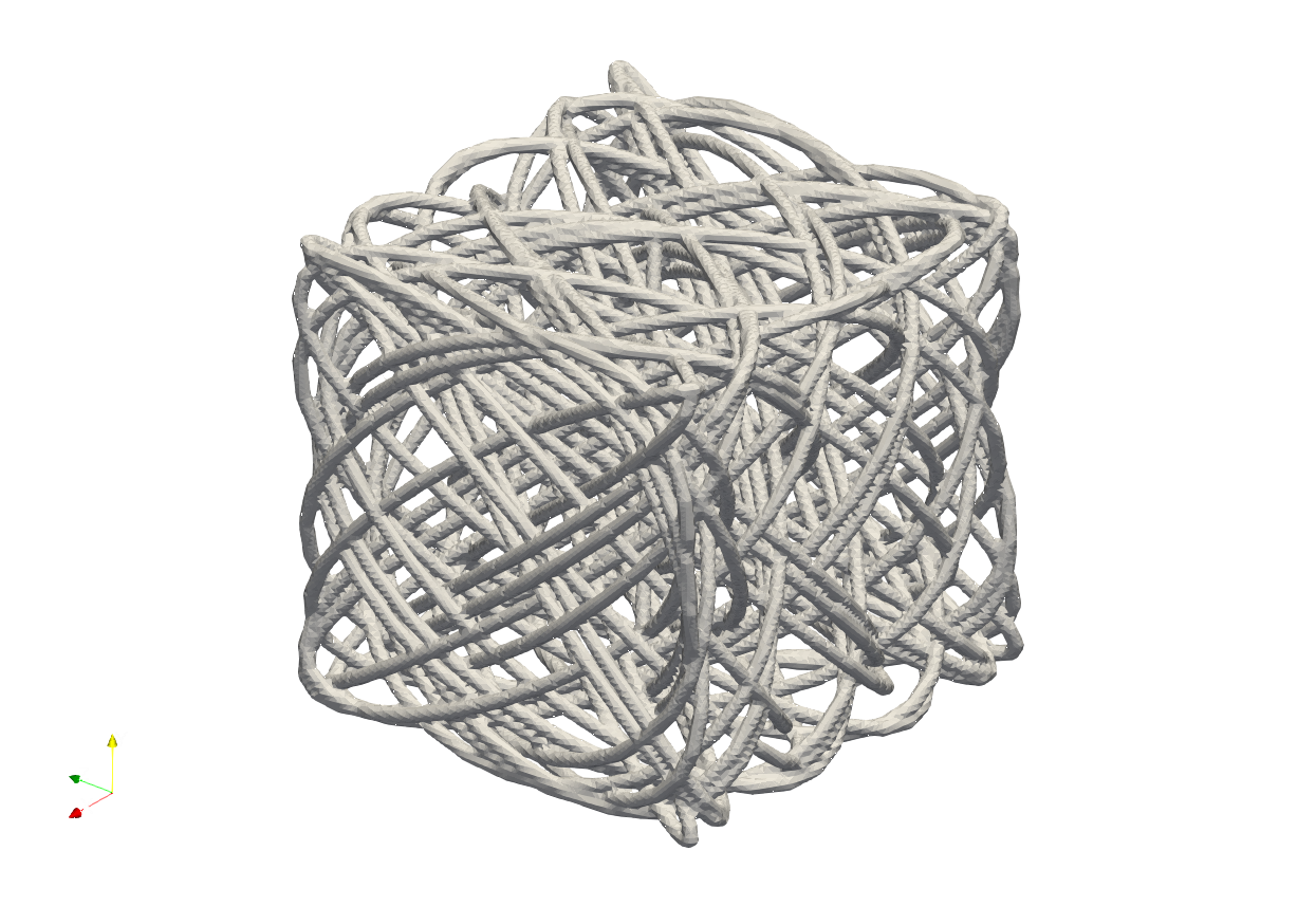
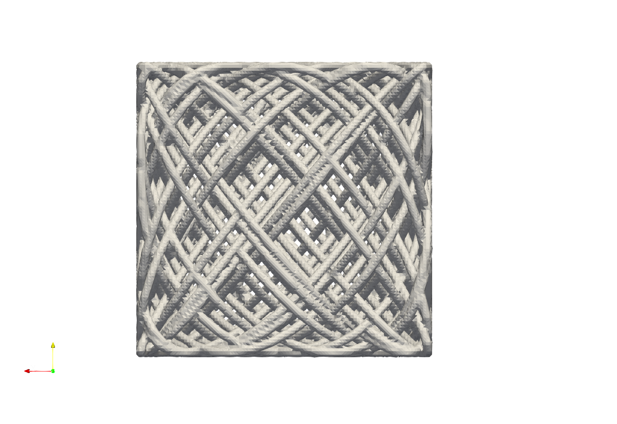
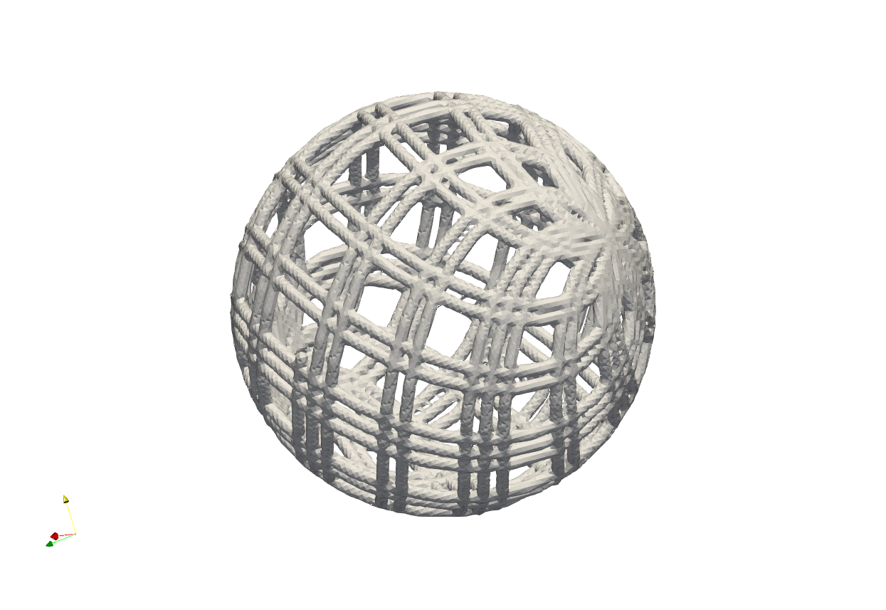
Example Test_jsonParametricGeometryParametricLines.json and Test_jsonParametricGeometryParametricLines_Sphere.json shows a complete workflow for a parametric curve filling a cubic volume and spherical volume.

Notes#

t_max must be greater than t_min.
At least one of n_points and step_size must be provided.
n_points must be at least 2.
step_size must be greater than zero.
The expressions must produce finite coordinate values over the entire parameter range.
The three expressions must define a curve rather than a single fixed point.
The generated mesh consists of line elements connecting consecutive curve points.

Line Structure 01

Contents

Line Structure 01#

Minimum Spanning Tree#

Streamlines over Field#

Parametric Curve#

Notes#